May 28th Bear
Creek Flash Flood Meteorological Analysis
By: Mike Evans
Flash flooding occurred in Bear Creek township in southeast Luzerne county late in the afternoon on the 28th as a mesoscale convective system developed across the area. New cells continually developed on the southwest flank of the system, then trained to the east across the flood area. The following figures show approximately 3 hours of radar imagery from the event. Note how storms continually formed on the southwest flank of the system, then moved east.
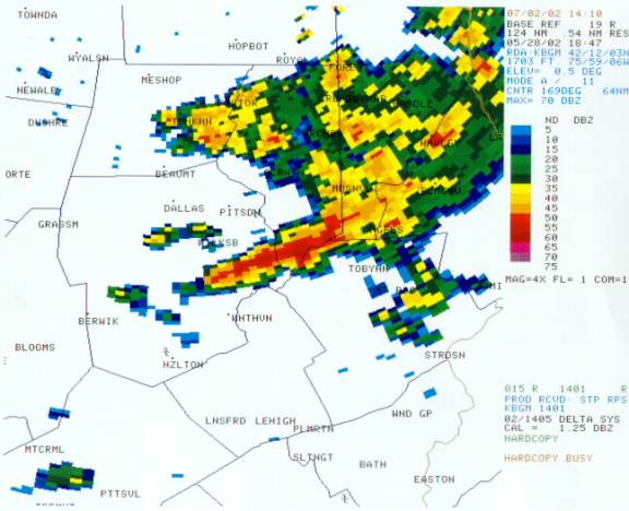
Radar imagery at 1847 UTC, May 28, 2002.
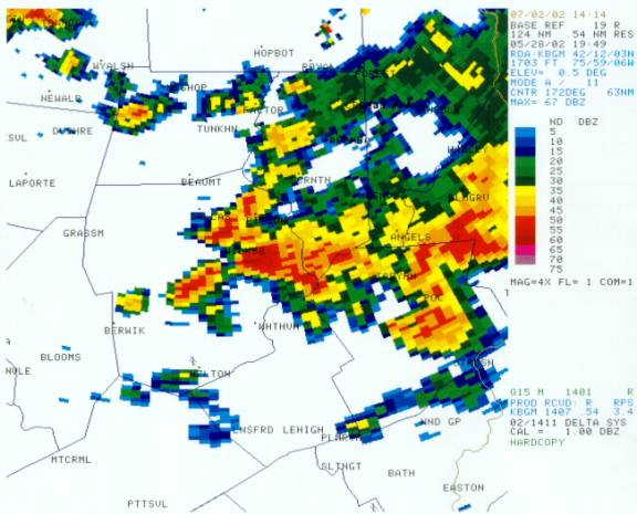
Radar imagery at 1949
UTC, May 28, 2002.
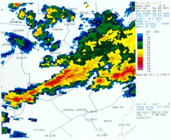
Radar imagery at 2049
UTC, May 28, 2002.
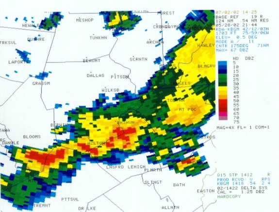
Radar imagery at 2144
UTC, May 28, 2002.
Radar estimates of total rainfall exceeded 9 inches in just a few hours before the storms finally moved south of the area.
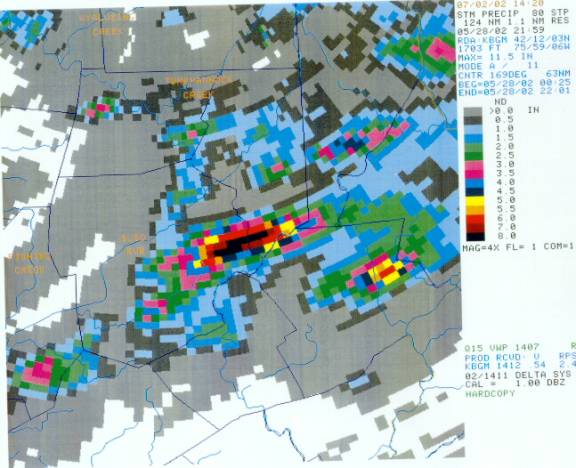
Storm total radar
estimated rainfall through 2159 UTC, May 28, 2002.
This event can be classified as a “frontal” type of flood event based on a classification scheme developed by Maddox in the late 1970s. In a “frontal” type of flood event, thunderstorms continually develop along a west to east oriented stationary or slow-moving warm front. The following figure shows a schematic of the environment characterized by “frontal” type flash flooding, as defined by Maddox.
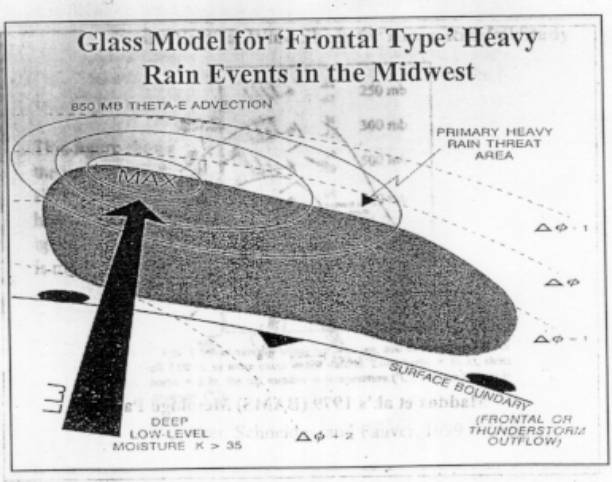
A schematic of the
environment associated with a Maddox “frontal” type flood. Note the low-level jet oriented
perpendicular to the surface frontal boundary.
The thunderstorms associated with this event could also be considered to be “backward propagating” in the sense that new storms continually developed southwest of the main convective system, then trained to the east, causing the flooding.
The following is a list of characteristics of the environment associated with a Maddox “frontal” type flood environment, accompanied by backward propagating thunderstorms.
1) The area is typically in the right entrance region of an upper level jet.
2) An east-west surface boundary is typically present.
3) Low-level jet: Normal to the upper level jet, normal to the surface boundary, and just upstream from the flooding MCS. The speed of the low-level jet is typically greater than or equal to 30 knots. A horizontally broad low-level jet is preferable to a narrow low-level jet.
4) A weak surface low-pressure area is typically located upstream of the flood.
5) A weak short wave is located upstream of the heavy rain.
6) Weak mid to upper level wind shear (weak 850-300 mb winds) is present.
7) Thickness diffluence is present.
8) Thickness saturation: climatological location of heavy precipitation based on the following table from Funk 1991: Use PW of the in-flowing air, 1000-500 mb thickness at the location of interest.
1000-500 thickness = 552 dm, PW=0.70
1000-500 thickness = 558 dm, PW=0.80
1000-500 thickness = 561 dm, PW=0.90
1000-500 thickness = 564 dm, PW=1.05
1000-500 thickness = 567 dm, PW=1.15
1000-500 thickness = 570 dm, PW=1.25
1000-500 thickness = 573 dm, PW=1.40
1000-500 thickness = 576 dm, PW=1.55
1000-500 thickness = 579 dm, PW=1.70
1000-500 thickness = 580 dm, PW=1.90
9) Maximum of CAPE is near or upstream from the MCS. Values of greater than 2000 J/kg are favorable.
10) Theta-e ridge along and upstream from the MCS.
11) The strongest low-level moisture convergence is located upstream from the MCS.
12) Warm cloud depth (T greater than 0C) is 3 km or greater.
13) Deep saturation; ie no significant dry layers in the soundings near the thunderstorms.
14) Long, narrow CAPE profiles are preferable to short, fat CAPE profiles.
15) Small MBE vectors, or MBE vectors parallel to the low-level boundary (along with the absence of dry air). The MBE vector is the vector difference between the mid-level flow, which steers the individual thunderstorm cells, and the opposite of the low level flow, which is an indication of where new cells will develop based on how the low-level flow interacts with the old cell’s cold pool. Small MBE vectors would indicate the potential for stationary areas of high reflectivity, while MBE vectors parallel to the low-level boundary would indicate the potential for training storms.
Note: Individual cell movement should not be confused with system movement. Often-times, individual cells within a large convective system will move in one direction, while the system of cells moves in another direction. MBE vectors predict the movement of the system, not individual cells.
Note: In uni-directional flow, the mid-level “system advection” vector will oppose the low-level “system propagation” vector, which can result in small MBE vectors and could imply slow cell movement. However, when dry air is injested into a storm, in a uni-directional flow regime, the movement of the individual cells and the MCS will often be very fast, in the direction of the flow, not in the direction of the smaller MBE vector. This is because in that case, the cold pool can become very cold relative to the surrounding air, and will tend to propagate quickly east in the direction of the mid-level steering flow. The best inflow relative to the cold pool (gust front) in that case will then be on the downwind side of the cold pool, causing the propagation vector to point in the same direction as the advection vector. A warmer cold pool favors a slower moving cold pool, in which case the best storm relative inflow toward the cold pool will be on the upwind side of the cold pool. The result is that the propagation vector would point upwind, opposing the advection vector, and resulting in a slower moving or upwind moving storm.
The rest of this case study will examine data from this event (primarily Eta 6-12 hour forecast gridded data and soundings), and compare the data to the rules listed above.
1) The region is typically in the right entrance region of an upper jet. This is a favorable area for upper-level divergence. The left-exit region is also a favorable area for upper divergence, however the best low-level moisture is typically located underneath areas south of the main jet, making the right entrance region most favorable for convective heavy rains during the warm season. In our case, northeast Pennsylvania was in the right entrance of an upper jet located east of Maine. It could also be argued that northeast Pennsylvania was in the left exit region of a jet over the southern Great Lakes area.
Eta 6 hr forecast 250
mb isotachs verifying at 5/28 18z.
2) An east-west surface boundary is typically present. The next two figures indicate that a weak west to east surface boundary was located across northern Pennsylvania during the afternoon on the 28th. This boundary may have been a combination of a synoptic scale front, and an outflow boundary left-over from convection that moved across southern New York state earlier in the morning.
Surface plotted winds,
temps and dew pts 5/28 19z.
Eta 3 hr forecast pmsl
verifying 5/28 15z.
3) A low-level jet oriented normal to the upper level jet, and normal to the surface boundary. The speed of the low-level jet is typically 30 knots or greater. A broad low-level jet is preferable to a narrow jet. The role of the southerly low-level jet is to transfer moisture and instability over the frontal zone. In addition, a southerly low-level jet will act to continuously develop new convective cells at the nose of the jet, as the jet interacts with the cold pools generated by previous convection. A broad low-level jet is preferable because it would be able to feed new cells across a relatively large area. In our case, we had a weak southerly jet extending up through 850 mb across eastern and central Pennsylvania. The forecast speed of the low-level jet was only 20 knots. It may be that the 30 knot rule was derived mostly in the Plains, where the low-level jet is often stronger than farther east. Also, keep in mind that a southerly flow across eastern Pennsylvania has a significant upslope component into the higher elevations of the Pocono mountains, where this flood occurred. Therefore, a lower speed may have been required than what would be needed over the Plains. The width of the low-level jet appears to have been approximately 150 miles or so, covering much of central and eastern Pennsylvania.
Eta forecast 850 mb isotachs verifying at 21z 5/28. Note the south to north maximum of around 20 knots indicated over eastern and central Pennsylvania.
Eta forecast cross
section of wind speed (kts) taken from Lancaster Pa, to Binghamton NY.
4) A weak surface low pressure system is typically located to the west of the flood. Our case had a weak low pressure system to the west, located over northern Ohio at 21z on the 28th.

Eta 09 hr forecast pmsl verifying 5/28/02 21z.
5) A weak short-wave at 500 mb is typically located upstream of the flood. Our case had this feature, located over central Pennsylvania at 18z.
Eta 06 hr forecast 500
mb height and vorticity verifying 5/28/02 18z
6) Weak mid to upper tropospheric winds with weak shear. In our case, the winds from 700 mb to 400 mb were from the southwest, gradually increasing with height from less than 10 knots at 700 mb to around 30 kts at 400 mb. The winds also increased with decreasing height below 700 mb, reaching around 15 to 20 knots with the low-level jet at 850 mb.
Eta bufkit forecast sounding at avp verifying 5/28/02 17z
7) Thickness diffluence. The following figure shows weak thickness diffluence across Pennsylvania at 21z on the 28th.
Eta forecast 1000-500 mb thickness verifying 21z 5/28.
8) Thickness saturation. Look for precipitable water values in the inflow region of at least the saturation value corresponding to the 1000-500 mb thickness in the area of interest. In this case, the thickness across northeast Pennsylvania was around 563 dm. Based on table shown earlier in this document, the saturation precipitable water for a thickness of 563 dm would be around 1.00 inches. The following figure shows the Eta forecast precipitable water for our case, indicating that downstream “inflow” values of around 1.3 inches. Based on the data from the table, this would be sufficient for a heavy rain event.
.
6 hr eta forecast precipitable water values verifying 5/28 18z.
9) Maximum CAPE is near or upstream of the flooding MCS with values of 2000 J/kg or greater. In our case, the Eta forecast CAPE values were around 1800 J/kg over central Pennsylvania, which would have been just upstream of the flood. Some heating in the warm sector just after this time could have resulted in CAPES of near or just over 2000 J/kg.
Eta 3 hr forecast CAPE verifying 15z 5/28.
10) A theta-e ridge along and upstream from the flooding MCS. This is obviously favorable since it would provide a source of maximum moisture for the MCS. In our case, there was a pronounced theta-e ridge at 850 mb, with its axis just to the west of the flooding MCS.
Eta 6 hr forecast 850 mb theta-e verifying 5/28 18z.
11) Maximum low-level moisture convergence and theta-e advection along and just upstream from the flooding MCS. In our case, Eta forecasts appeared to forecast an area of low-level convergence and theta-e advection just to the north of its low-level front, across southern New York. However, radar loops (not shown) from earlier in the day indicate that convection moved from southern New York southeast across northeast Pennsylvania during the morning and early afternoon on the 28th. (The convection lead to flooding earlier in the morning in the Binghamton area). As a result, outflow boundaries from that convection were likely located over northeast Pennsylvania, which would have made the low-level boundary farther south than what the Eta model was depicting on its 12z forecasts.
Eta forecast 850 mb
theta-e convergence verifying 5/28 18z.
12) A warm cloud depth of 3 km or greater. This is favorable, since warm cloud rain producing processes tend to be most efficient at producing heavy rain. In our case, the warm cloud depth appeared to be only around 2 km.

Eta bufkit forecast sounding at AVP verifying 5/28/02 17z.
13) Deep saturation; ie no significant dry layers in the forecast soundings. None of the soundings in our case appear to exhibit any significant dry layers.
14) Profiles with long, narrow CAPE are more favorable for heavy rain and flooding then profiles with short, fat CAPE. A deep layer of CAPE will produce a very tall thunderstorm, which is best for precipitation efficiency. Short, fat profiles of CAPE will produce very strong updrafts, but the storms will not be as tall. This would be more favorable for severe weather than for heavy rain. In our case, all of the forecast soundings along and south of the front exhibited narrow, deep CAPE profiles.
15) Small MBE vectors, in the absence of dry air, are favorable for individual cells to remain nearly stationary, or sometimes to even track just upstream from their initial development points. MBE vectors parallel to the low-level boundary can result in cells continually training along the boundary. Either situation can be favorable for heavy rain. Recall that an MBE vector is the vector difference between the mid-level flow vector, which steers the individual cells, and the opposite of the low-level flow vector, which dictates where new cell development can be expected based on how the low level flow will interact with the old cell’s cold pool. In our case, the MBE vectors were not that small, and pointed toward the southeast (the mid-level flow vector pointed toward the east, and the opposite of the low-level flow vector pointed toward the south. The resultant MBE vector pointed southeast). This would imply that the individual cells in our case should move southeast. However, the key to this event, was that while the individual cells tended to move east, the entire system remained anchored as new cells continually reformed upstream from the old cells. This was most likely the result of new cells forming in response to the low-level jet interacting with the nearly stationary frontal boundary, plus the effect of the low-level jet being oriented in a direction that was “upslope” relative to the rising terrain in the southern Pocono mountains.
Eta Bufkit AVP forecast sounding verifying 5/28 18z. Note the MBE vector pointing toward the southeast (blue arrow).
SUMMARY:
The flash flood event of 5/28/02 in northeast Pennsylvania exhibited many of the characteristics of a classic Maddox “frontal” type flash flood event. A few aspects from this case that were less than classic was the relatively weak low-level jet, forecast at only around 20 kts at 850 mb. The forecast warm layer cloud depth of 2 km was also a bit less than what might be expected for a warm season flash flood environment. Aspects of this event that were typical of “frontal” flash flood type environments included the presence of an east-west surface frontal boundary under the right entrance of an upper jet, sufficient instability and moisture on the warm side of the boundary, and a topographic feature that helped to anchor the convection.