January 19^th, 2002

INTRODUCTION / LARGE SCALE FORCING

Our system of interest was a relatively weak surface low pressure system moving northeast off of the mid-Atlantic coast. The system appeared to be located in the right entrance region of a 300-mb jet maximum moving east across New England. There did not appear to be a second, southern branch upper-level jet. The flow was of relatively low-amplitude, without any major upper level troughs. The surface pmsl, 300 mb heights and isotachs, and 700 mb heights shown below are all 9 hour forecasts from the Eta model verifying at 21z on the 19^th.

Surface pmsl and 850 mb temperatures

300 mb heights and wind speed.

Eta 09 hr forecast 700 mb heights verifying at 1/19 21z.

The following figure shows a 12 hr eta forecast of potential vorticity in the layer from 500 to 300 mb, verifying at 1/19 21z. The main lobe of PV is shown back across the western Ohio Valley, with only a weak eastward extension shown farther east across the mid-Atlantic region.

09 hr eta forecast 500-300 mb PV verifying 1/19 21z.

The large-scale geostrophic forcing for upward motion in this case can by implied from the following figure. Divergence of Q vectors is shown in the layer from 500 to 400 mb. Recall that upward motion is favored in areas where the divergence is negative. Recall also that the vertical motion implied by the divergence of Q does not include the effects of stability, which in the real atmosphere are significant (instability increases vertical motion given equal forcing). In addition, the divergence of Q will not do a good job capturing the details of the vertical motion field in locations where there are strong ageostrophic winds, ie near fronts and jet streaks. In a case like this, where fronts and jet streaks are important, the divergence of Q cannot accurately predict the total vertical motion field, instead it should be thought of as depicting the “large-scale” forcing for vertical motion. In this case, a very weak, banded pattern of forcing is indicated across Pennsylvania and New York State. This is an indication that the forcing for the snow band in question was probably not “large-scale”, but was associated with smaller scale features (such as a front or jet streak).

09 hr eta forecast 500-400 mb divergence of Q verifying 1/19 21z.

The patterns shown above resulted in relatively narrow, weak bands of upward vertical motion and saturation. The figure below shows the mean layer vertical velocity and relative humidity from 600 to 500 mb, verifying at 1/19 21z. Note that the vertical velocity shown in this figure is the total model forecast vertical velocity, and includes the effects of stability and ageostrophic flow. The vertical motion fields are still fairly weak, but at least they indicate a maxima in the area where the heavy snow band developed.

09 hr eta forecast 600-500 mb layer average omega and rh verifying 1/19 21z.

MODEL QPF VS OBSERVATIONS

Radar loops indicated that a band of moderate to heavy snowfall developed on the northern edge of the system across northern Pennsylvania and southern New York during the afternoon on the 19^th. The band eventually weakened and pivoted to the southeast during the evening.

Since the band eventually pivoted southeast across Pennsylvania, QPF totals across Pennsylvania and southern New York were fairly uniform. However, very high snow to liquid ratios over southern New York resulted in an unexpected 6 to 12 inch snowfall across southern New York, despite an average of only around 0.25 inches of liquid in that area. The following figure shows the total observed precipitation for this event (mm) through 1/20 00z. Note that the movement of the band resulted in an even distribution of precipitation from southern New York through Pennsylvania.

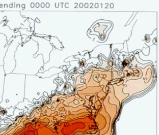
Observed precipitation (mm) through 1/20 00z.

Observed snowfall through 1/20 06z. Note the band of 8 to 12 inches of snow across the southern tier of New York.

The BUFKIT Eta forecast sounding shown below indicates that southern New York had a somewhat unusual temperature profile for a snowstorm during this event. Note that the lack of strong QG forcing associated with this event meant that there were no layers of strong warm advection, and therefore no pronounced warm layers in the forecast sounding. As a result the sounding was roughly moist adiabatic through a deep layer. The result was a favorable temperature (around –15 degrees C) for snow growth by deposition in the mid-levels of the sounding, combined with a favorable temperature (just below 0 degrees C) for crystal growth by aggregation in the lower levels of the sounding.

The following figure is a time cross section of Eta forecast temperature and relative humidity at BGM. Note the long period where high relative humidity values combined with a deep layer of near –15 degrees C across the area.

BUFKIT depiction of Eta forecast relative humidity and temperature at BGM.

MODEL DIAGNOSTICS

1) FORCING FOR UPWARD MOTION

A 9 hour eta forecast of 850 mb moisture convergence verifying at 1/19 21z indicates a strong maximum over the Delmarva peninsula area, where the southern area of heavy precipitation occurred. Enhanced southerly flow occurred in this region where there was a strong low-level gradient of temperature and moisture, resulting in moisture convergence, upward motion and precipitation.

850 mb moisture convergence and 850 mb wind barbs at 21z on the 19^th.

However, looking at only level when trying to diagnose the potential for upward motion can be deceiving. Note that little if any forcing is indicated across northern Pennsylvania and southern New York by this figure.

The following figure shows a cross section of frontogenesis from Philadelphia to Rochester for 21z on the 19th. The frontogenesis slopes upward from south to north across the region. Note a strong maximum located along the southern part of the front, and a secondary maximum located to the north, near the heavy snow band. Reasons for this double maximum will be explored later.

Cross section of frontogenesis (frnt(tmpc,obs)) at 21z on the 19^th. The cross section is from PHL to ROC.

A plan view of frontogenesis at 625 mb at 21z on the 19^th shows that the frontogenesis at that level lines up very well with the location of the snow band.

Frontogenesis at 625 mb at 21z 1/19.

The components of frontogenesis can be clearly seen on the next two figures. The first figure shows 625 mb stretching deformation and wind barbs, as forecast by the Eta at 21z 1/19. The second figure shows the 625 mb forecast temperature in degrees C. Note that the area of maximum deformation corresponds to an area of enhanced temperature gradient over southern New York. The axis of dilatation implied by the wind barbs would be roughly parallel to the isotherms, indicating strong frontogenesis. Finally, note how well then –15 degree C isotherm lines up with the band of heavy snow shown in earlier figures.

Stretching deformation and wind barbs at 625 mb, 1/19 21z.

Temperature (degrees C) at 625 mb at 21z 1/19.

The stretching deformation maximum across northern Pennsylvania and southern New York was caused by confluence between a southwesterly flow across Pennsylvania and a more westerly flow farther to the north. The next figure shows ageostrophic wind barbs and heights at 625 mb verifying at 1/19 21z

Ageostrophic wind barbs and heights verifying 1/19 21z.

The strong southeasterly ageostrophic flow over Pennsylvania apparently resulted in a confluent (and convergent) flow across northern Pennsylvania and southern New York. The combination of confluence and the ambient temperature gradient resulted in the frontogenesis maximum. For insight into what caused the strong ageostrophic southeast flow, consider the next two figures. In the first figure, 500 mb isotachs are shown, along with 500 mb divergence. Note the strong speed maximum approaching the area from the southwest. Pennsylvania and southern New York are in the left exit region of this speed maximum. The thermally indirect circulation in the exit region is indicated by the divergence in the left exit region over Pennsylvania and southern New York, and by the ageostrophic southeast flow below the exit region shown in the proceeding figure. In the second figure, ageostrophic wind barbs and heights are shown at 500 mb. Note that, in contrast to the first figure, the ageostrophic flow is from the north across southern New York and Pennsylvania. The figure taken at 625 mb appears to be showing a view of the lower branch of the circulation, while the figure taken at 500 mb appears to be showing a view of the upper branch of the circulation.

500 mb isotachs (shaded) and divergence verifying at 1/19 21z.

500 mb heights and ageostrophic wind barbs, verifying 1/19 21z.

A cross section of forecast omega and frontogenesis indicates a maximum of upward vertical motion located just above the axis of maximum of frontogensis. The upward vertical motion maximum is fairly shallow, extending along and just above the frontal zone.

Frontogenesis (black lines) and omega (purple lines).

One interesting aspect of this event appears to be that the upward motion associated with the event was quite shallow. Note that a sloping band of subsidence appears just above the upward motion maximum associated with the frontal boundary. Another band of upward motion then appears above this subsidence, in the upper levels of the troposphere.

The figure below shows the relationship between the location of the maximum of upward vertical motion and wind speed. Note again that the band of upward vertical motion maximum is fairly shallow.

Cross section of omega and isotachs verifying at 1/19 21z.

A cross section of divergence and wind speed taken along the same line from PHL to ROC shows the relationship between divergence, the location of the frontal zones, and the upper level jet. As would be expected, upward motion is forecast in areas where convergence changes to divergence with height. Also, note that areas of low-level convergence indicate the location of the low-level frontal zones. The data in the following figure indicate that there are really two frontal zones associated with this event, a mid-level front across the north located underneath the upper level jet, and a low-level front farther to the south. Convergence and frontogenesis maxima are associated with both fronts.

Eta 12 hour forecast of divergence (black lines) and wind speed (purple lines) from PHL to ROC verifying at 1/20 00z.

A cross section taken along a longer line, from ORF to ROC, better shows the structure of the upper jet. Note that the speed max at 500 mb is really just part of a single jet that slopes southwestward from above 300 mb down through 500 mb. In this figure, the jet not only slopes downward from left to right, but also slopes downward out of the page. As a result, this cross section is taken in the exit region of the jet around 500 mb, and in the entrance region of the jet at 300 mb. The sloped band of divergence between 400 and 700 mb is associated with the left exit region of this sloped jet, while the divergence farther up in the troposphere is associated with the right entrance region of the same jet at upper levels.

Isotachs (black lines) and divergence (purple) verifying at 1/19 21z.

2) ASSESSING INSTABILITY

An Eta forecast cross section of frontogenesis and theta, taken from PHL to ROC and verifying at 1/19 21z is shown below. Note the frontal zone sloping from south to north. The double maximum of frontogenesis is indicated, with a weaker maximum located to the north near the heavier snow band. An area of weak stability is located above the band of frontogenesis (indicated by the theta lines being spread relatively far apart).

The following figure shows a cross section of theta-e and momentum, taken across the frontal zone along a line from PHL to ROC at 1/19 21z. Note the narrow band of potential symmetric instability (PSI), in the zone just above the frontal zone, where the theta-e lines slope more steeply than the momentum lines. In fact, the theta-e lines appear to “fold over” on themselves in this case, indicating the presence of conditional instability, especially over the central and southern part of the cross section. In the area above northern Pennsylvania and southern New York, the atmosphere appears to be just about neutral.

A cross section of theta-e and momentum, taken from PHL to ROC and verifying 1/19 21z.

A cross section of frontogenesis and EPV indicates that a narrow band of negative EPV was associated with this band of PSI (and conditional instability). Again, note that this band of weak stability is located just above the frontal surface.

A cross section of frontogenesis (black lines) and EPV (purple lines, only negative values are plotted). Note the band of negative EPV located just above the sloping band of frontogenesis.

The following figure shows a cross section of negative EPV and relative humidity, verifying at 1/19 21z. Note that the negative EPV occurs along the vertical saturation gradient, with high values at the bottom of the negative EPV zone, and low values at the top.

A 12 hr eta forecast of EPV (only negative values plotted) and relative humidity, verifying at 1/19 21z.

The following figure shows the relationship between vertical velocity and negative EPV for this case. The negative EPV layer is located within a zone of upward vertical velocity.

12 hr eta forecast of vertical velocity and epv (only negative values plotted) verifying at 1/19 21z.

The proceeding figures indicate that a layer of conditional instability developed above a sloping frontal zone in this case. The layer was shallow, but located in a position where the upward motion associated with the large scale dynamics of the system, as well as the circulation induced by frontogenesis became co-located with the instability. The result was that the circulation associated with the mid-level frontogenesis became strengthened and localized, leading to the intensification of the snow band.

A cross section of theta-e advection taken from PHL to ROC shows positive advection along the frontal boundary with weak negative advection above in the southwest flow. The result is decreasing stability above the frontal boundary. This differential advection of theta-e is apparently responsible for the development and maintenance of the instability shown in the previous few figures.

Cross section of theta-e advection. Note the positive values below and especially along the frontal boundary, with negative values above the front. The result is decreased stability above the front.

Summary:

This is an interesting an event from several perspectives. Despite the fact that the QPF with this event was fairly even distributed across Pa and southern New York, radar loops indicate that the event was characterized by a fairly narrow band of moderate to heavy snow. The band eventually moved across a large area, resulting in the even distribution of QPF. Despite the even distribution of QPF, the snowfall amounts varied widely. It is hypothesized that the main reason for the heavy snow falling over northern Pennsylvania and southern New York was a favorable temperature profile across that area. Farther south, the temperature profile was warmer, and not as favorable for snow growth.

The mechanisms that produced the narrow, heavy band of snow with this case are another interesting aspect of the case. The moderately heavy precipitation that fell over the Delmarva peninsula to the south of the band apparently were associated with strong low-level moisture convergence and lift along a strong, low-level baroclinic zone. The moderate to heavy precipitation in a narrow band farther to the north was apparently generated by frontogenesis and convergence that developed along a second, northern frontal zone located directly underneath the upper-tropospheric jet. Vertical motion was maximized above this second northern frontal boundary as 1) an area of divergence associated with the left-exit of a 500 mb speed maximum moved over the top of the jet (the speed maximum was associated with a single, sloping jet stream which sloped downward from the northeast toward the southwest), and 2) the area above the front became destabilized due to strong differential theta-e advection associated with a dry slot advancing eastward across the area in the moderately strong southwesterly flow. (This instability would have acted to intensify and focus the lift along the axis of frontogenesis).

As far as Phil’s ideas regarding narrow, heavy snow bands on the northern edge of systems: this system appeared to be similar to the case in South Dakota in that there was no coupled jet circulation in evidence. In Phil’s case, two jets were present; they were just too far apart to be coupled. In this case, there was apparently only one jet, so no coupling could occur. Like in Phil’s case, this was a case where the flow was relatively straight (ie no major upper level trof). As a result, upward motion generated by changes in wind speed along the flow (jet streaks) would be allowed to dominate the upper level divergence fields, without interference from curvature effects.

An important aspect that determined the configuration of the precipitation echoes with this event was the lack of strong, widespread forcing that would typically be associated with a deep mid to upper level trough. When a deep mid to upper level trough is present, curvature effects associated with the upper level flow result in large scale upward motion forcing and large areas of light to moderate precipitation. In this case, the upward motion was confined to the areas where vertical motion associated with mid-level frontogenesis, in combination with instability, acted to produced a more localized area of moderate precipitation.

PHL

BGM

Maximum of upward motion

(best isentropic lift)

500 mb jet exit region (jet into page)