WFO BGM LOCAL CASE STUDY ON THE FEBRUARY 17, 2003
(PRESIDENT’S DAY) SNOWSTORM
1. Introduction
Heavy snow fell across most of central New York and northeast Pennsylvania during the day on the 17th, as low pressure moved east off of the mid-Atlantic coast. In section 2 of this case study, a quick review of radar imagery, snowfall reports, and basic weather maps will be shown. In section 3, the mechanisms responsible for producing the heavy snow will be examined in more detail. Observations and forecasts from the Eta and GFS models will be compared and contrasted. Section 4 contains a brief summary and conclusions.
2. Observations and Basic Weather Maps
Snow began falling across northeast Pennsylvania during the predawn hours on the 17th, then spread north to cover all of central New York by late morning. The snow ended from south to north late Thursday afternoon and Thursday night. Snow accumulations averaged around a foot across most of the area, with localized heavier amounts of up to 2 feet reported from northeast Pennsylvania east to Sullivan county, New York. Figure 1 shows a map of snowfall reports from the storm.
Figure 1. Observed
snowfall totals from the Presidents Day Storm.
The data in Figure 1 shows a maximum snowfall of 27 inches over Sullivan county, however most of the area received anywhere from 8 to 14 inches of snow.
Figures 2a through c show radar images from the KBGM WSR-88D Doppler radar.
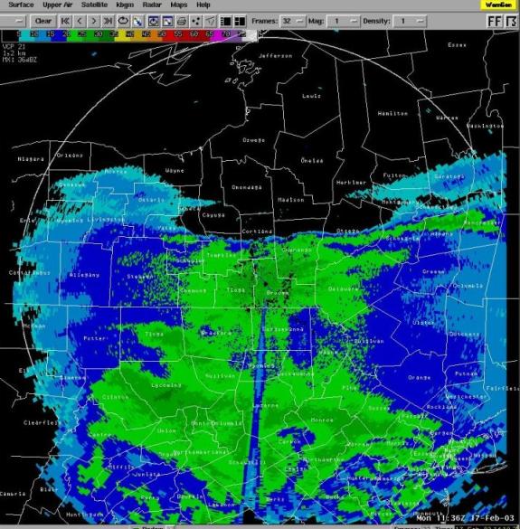
Figure 2a) Snow
beginning to overspread south central New York, from the south during the
morning on the 17th.
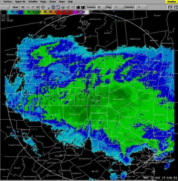
Figure 2b) Snow covers
most of northeast Pennsylvania and central New York during the afternoon on the
17th.
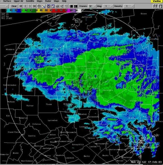
Figure 2c) Snow begins
to end across northeast Pennsylvania late in the day on the 17th, as
the main band of snow lifts off to the north.
These figures indicate that a wide band of moderate to heavy snow lifted north across the area during the 17th. Unlike the Christmas 2002 storm, no narrow bands of extremely heavy snow were indicated, however most of the area experienced several hours of moderate snow with accumulations averaging around an inch an hour for several hours.
Figures 3 through 5 show Eta forecasts of 250 mb wind speed, 500 mb heights, and mean sea-level pressure verifying at a) 1800 UTC on the 17th and b) 0000 UTC on the 18th.
Figure 3a) 00-hour Eta
forecast 250 mb wind speed verifying at 2/17 1200 UTC.
Figure 3b) 12-hour Eta
forecast 250 wind speed verifying at 2/18 0000 UTC.
Figure 4a) 00-hour Eta
forecast 500 mb heights verifying at 2/17 12 UTC.
Figure 4b) 12-hour Eta
forecast 500 mb heights verifying at 12/18 0000 UTC.
Figure 5a) 00-hour Eta
forecast mean sea-level pressure verifying at 2/17 1200 UTC.
Figure 5b) 12-hour Eta
forecast mean sea-level pressure verifying at 2/18 0000 UTC.
Pennsylvania and New York appeared to be in the left exit region of a jet streak moving northeast off of the east coast of the United States during the storm. The area may also have been in the right entrance region of a second jet streak moving east of New England at the beginning of the event. At 500 mb, the main upper-low center was located well to the west of the area, remaining over the Ohio Valley. At the surface, a weak area of low pressure was located over the west slopes of the central Appalachian mountains, while a secondary low pressure area developed east of the Carolinas and moved northeast to the south of Long Island. The low did not deepen rapidly, and in fact only reached a central pressure as low as 1008 mb by 0000 UTC on the 18th. However, a very strong surface high-pressure center (central pressure around 1038 mb) was located over eastern Canada, resulting in a strong easterly pressure gradient between the low to the south and the high to the north.
- Forcing
for upward motion
As was the case for many of the major snowstorms during the 2002-2003 winter season, large differences in the precipitation forecasts were noted between the Eta and GFS model across central New York and northeast Pennsylvania, with the Eta model forecasting much more precipitation over the northwest quadrant of the storm. Figure 6a shows the 18-hour precipitation forecast from the Eta run at 12 UTC on the 17th, verifying at 06 UTC on the 18th. Figure 6b shows the 18-hour precipitation forecast from the GFS run at 12 UTC on the 17th and verifying at 06 UTC on the 18th.

Figure 6a.
18-hour precipitation forecast from the 12 UTC February 17th
run of the Eta model, verifying at 06 UTC on the 18th.
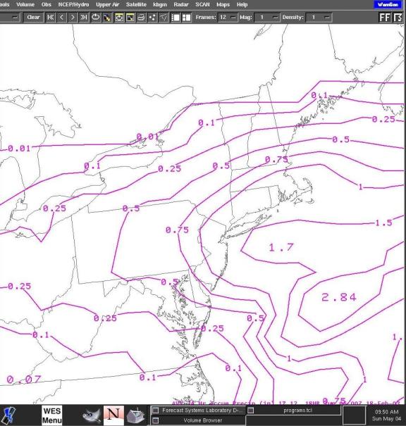
Figure 6b. 24-hour qpf
from the GFS verifying at 0600 UTC on the 18th.
The data in Figure 6a indicates that the Eta forecast between 1 and 1.5 inches of liquid equivalent precipitation across northeast Pennsylvania and between 0.5 and 1.0 inches of liquid equivalent precipitation across central New York. Snow to liquid ratios of approximately 15 to 1 based on this forecast would have resulted in snowfall amounts very to similar to what was observed. By contrast, figure 6b indicates that the GFS forecast between 0.50 and 0.75 inches of liquid over northeast Pennsylvania and between 0.25 and 0.50 inches across central New York.
Figure 7a shows Eta 6-hour forecasts of the large-scale forcing for upward motion (the 300-500 mb q-vector convergence) and the model total omega field, verifying at 1800 UTC on the 17th (the peak of the storm across our area). Figure 7b shows the same data, except from the GFS model.
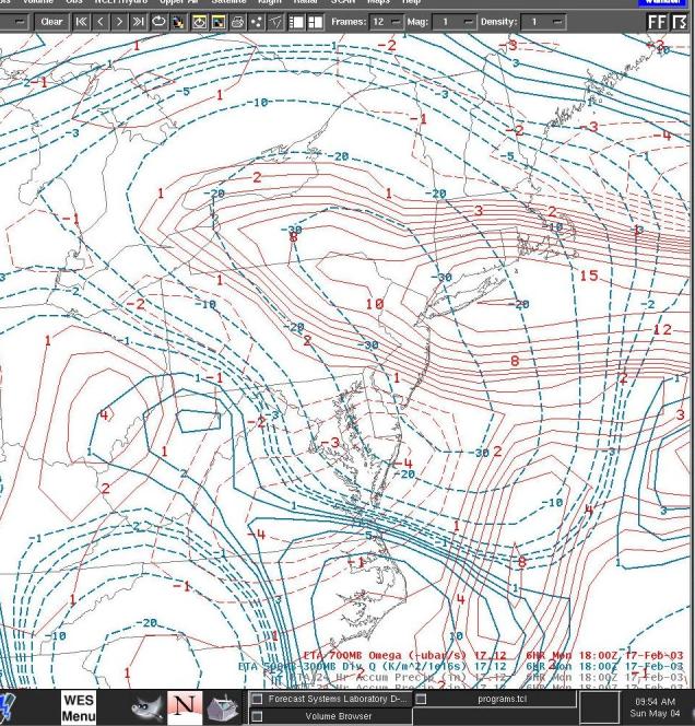
Figure 7a. 6-hour Eta forecasts of 300-500 mb q-vector convergence (dashed green lines) and model total omega (thin orange) lines.
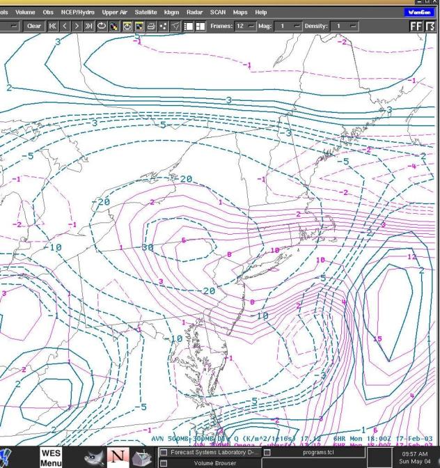
Figure 7b.
6-hour GFS forecast of 300-500 mb q-vector divergence (green lines) and
700 mb omega (purple lines) verifying at 1800 UTC on the 17th.
These figures indicate that both the Eta and GFS were forecasting the large-scale and total omega to be maximizing over the northern mid-Atlantic region during the mid-afternoon on the 17th. The large-scale forcing pattern exhibited an oval-shaped maximum across the northern mid-Atlantic region, while the total model omega indicated a more narrow, elongated east-to-west band of maximum values extending from southern New England east toward central New York and northern Pennsylvania. The Eta maximum forecast omega in our area was around 10 mb/s over extreme northeast Pennsylvania, while the GFS maximum forecast omega was between 6 and 8 mb/s over the same area.
The large-scale forcing for upward motion over New Jersey and eastern Pennsylvania was being driven primarily by a strong short-wave trough was rotating northward up the east coast around the large upper-level low-pressure area centered over the Ohio Valley. Figure 8a shows a plot of 6-hour Eta forecast 300-mb vorticity, wind and divergence associated with this short-wave. Figure 8b shows the same data, except for the GFS model.
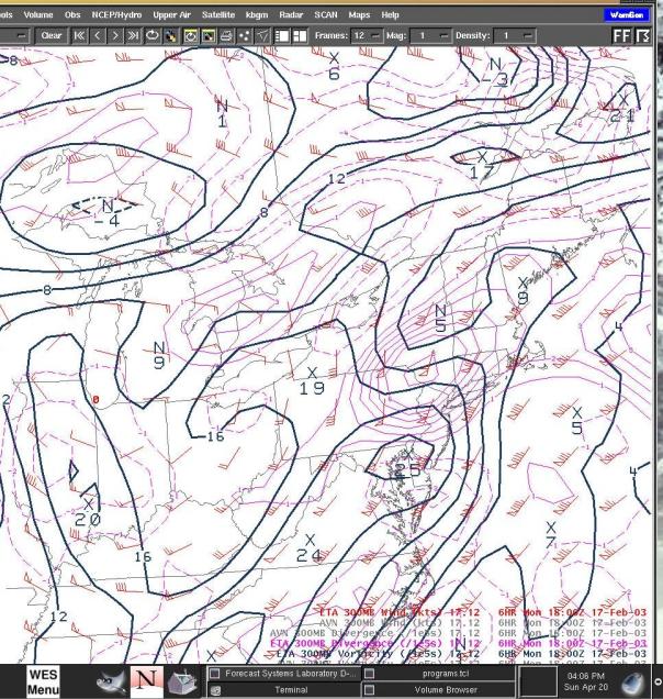
Figure 8a. 6-hour Eta 300-mb vorticity (black lines),
wind and divergence (purple lines) verifying at 1800 UTC on February 17th.
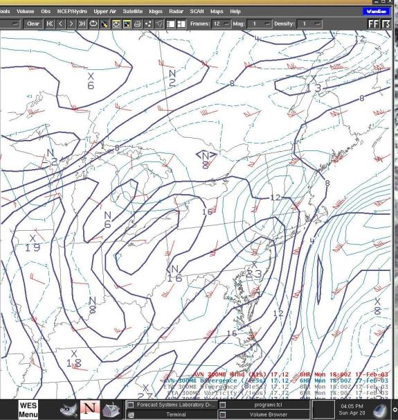
Figure 15. 6-hour GFS
forecast of 300-mb vorticity, wind and divergence verifying at 1800 UTC on the
17th.
Both models forecast a strong vorticity maximum (indicating the location and intensity of the short-wave trough) near Philadelphia, with a pronounced vorticity minimum (indicating the location and intensity of a downstream short-wave ridge) to the north. The Eta had a larger maximum and a much smaller minimum, indicating a stronger short-wave trough, and a much more pronounced downstream short-wave ridge. In addition, the separation between the implied trough and ridge was smaller on the Eta. Both models forecast a strong wind flow across the vorticity gradient, indicating upper-level vorticity advection, however the stronger vorticity gradient indicated by the Eta resulted in more vorticity advection and more upper-level divergence. The upper-level divergence forecast by both models corresponded well to each model’s maximum of
q-vector convergence, indicating that this was a significant contributor to the large-scale forcing for upward motion.
In this case, there was a significant difference between the shape of the large-scale forcing and the total model omega, indicating that the total forcing was likely being influenced by a significant, elongated contribution to the upward motion by smaller-scale forcing, probably associated with frontogenesis.
Figure 9 shows a 6-hour Eta forecast of 700-mb
frontogenesis, verifying at 1800 UTC on the 17th.
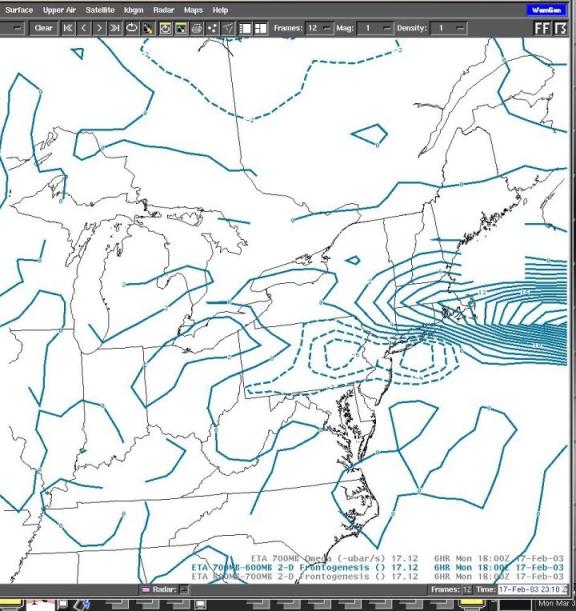
Figure 9. 6-hour Eta forecast 700-mb 2-D
frontogenesis, verifying at 1800 UTC on the 17th.
The data on Figure 9 indicate that the strongest mid-level frontogenesis at this time was located over eastern New England. Note that there was also a pronounced mininum of frontogenesis (frontolysis) located over eastern Pennsylvania. A strong gradient between the frontogenesis and the frontolysis was located across the area from northeast Pennsylvania through southern New England. Maximum vertical motion in a layer typically occurs on the warm side of the frontogenesis, or on the cold side of frontolysis, as an ageostrophic circulation develops to maintain thermal wind balance. In a case with frontolysis to the south and frontogenesis to the north, the strongest upward motion should occur in the gradient between the frontolysis and the frontogenesis. Figure 10a confirms that relationship, showing the Eta forecast total model omega and the frontogenesis at 700 mb. Figure 10b shows the same data, except for the GFS model.
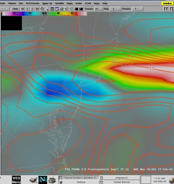
Figure 10a. 6-hour Eta forecast 700 mb frontogenesis
(image) and 700-mb omega (red lines) verifying at 1800 UTC on the 17th.
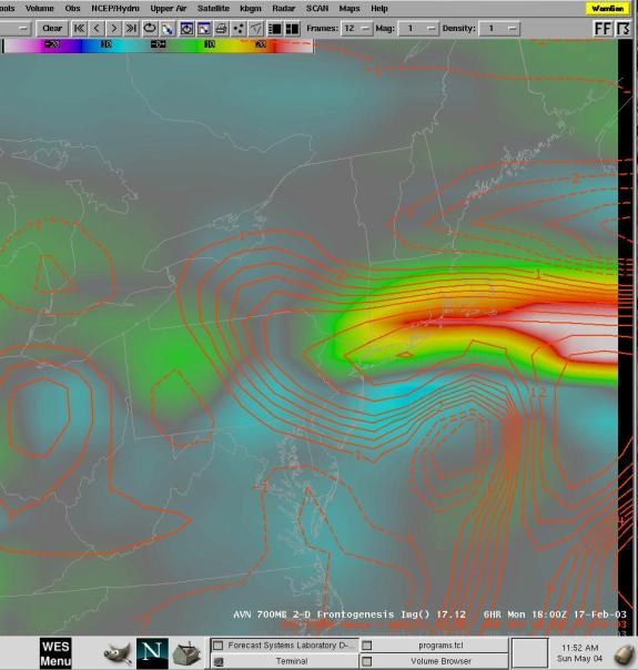
Figure 10b. 6-hour GFS
forecast of 700-mb frontogenesis (image)
and omega (red lines) verifying at 1800 UTC on the 17th.
Note that the elongated maximum in upward motion forecast by both models corresponds nicely to the strong gradient between the maximum of frontolysis over Pennsylvania and the maximum of frontogenesis over eastern New England.
The large circulation that developed across the mid-Atlantic states during the afternoon on the 17th was associated with strong upward motion across the northern mid-Atlantic states and a strong southeasterly low-level flow feeding moisture into the upward motion branch of the circulation from the western Atlantic. Figure 11a shows the Eta forecast 850 mb wind forecast, along with the 850 mb divergence, verifying at 1800 UTC on the 17th. Figure 11b shows the same data, except from the GFS model forecast.
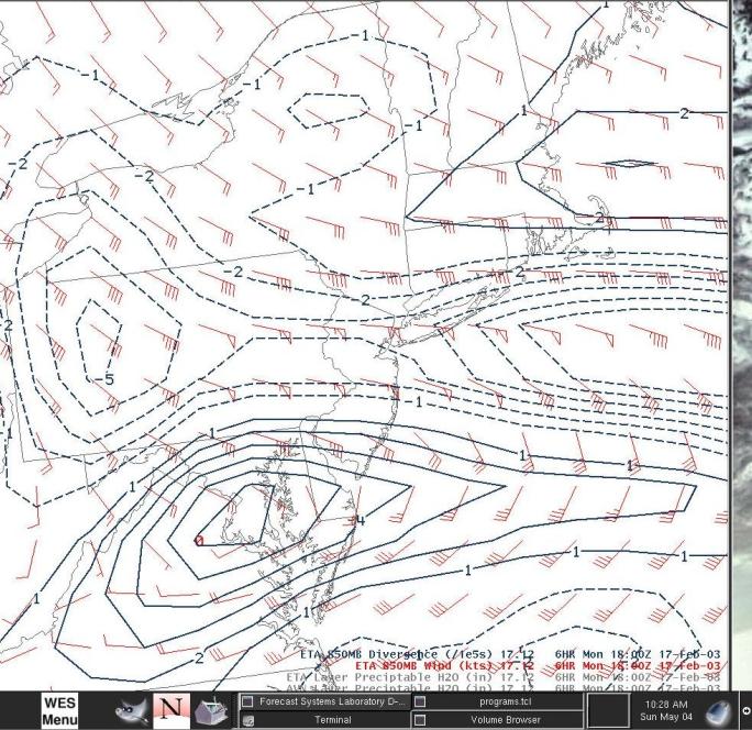
Figure 11a. 6-hour Eta 850 mb wind and divergence at
1800 UTC on the 17th.
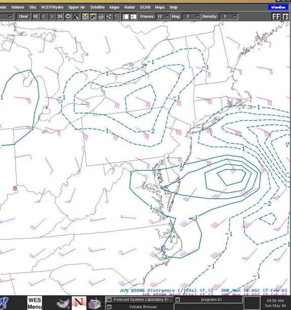
Figure 11b.
6-hour GFS forecast of 850 mb wind and divergence verifying at 1800 UTC
on the 17th.
Note that the Eta was forecasting 850 mb wind speeds to reach 60 kts from the east near New York City, with speeds dropping off to around 40 knots over central and western New York and Pennsylvania. The result was a strong band of convergence extending well inland across New York and Pennsylvania. Meanwhile, the GFS model was forecasting 850 mb wind speeds of around 40 kts near New York City, dropping off to around 30 kts over northern Pennsylvania and western New York. The resulting convergence over northern Pennsylvania and western New York was less in the GFS than the Eta. Figure 11c shows a time series of observed winds from the Brookhaven profiler on the 17th.

Figure 12. Wind data from the New Brunswick profiler on
February 17th, 2003.
The data from Figure 12 indicates that low-level easterly winds reached speeds of 50 to 55 kts during the 17th. This data indicates that the Eta did a good job forecasting the low-level easterly flow with this system, while the GFS forecast may have been a bit underdone. RAOB data from Brookhaven (not shown) also indicates that observed wind speeds were between 50 and 60 kts from the east at 850 mb.
Figure 13a shows a 6-hour Eta forecast of wind and pressure on the 295 K isentropic surface, verifying at 1800 UTC on the 17th. Figure 13b shows the same data, except from the GFS model forecast.
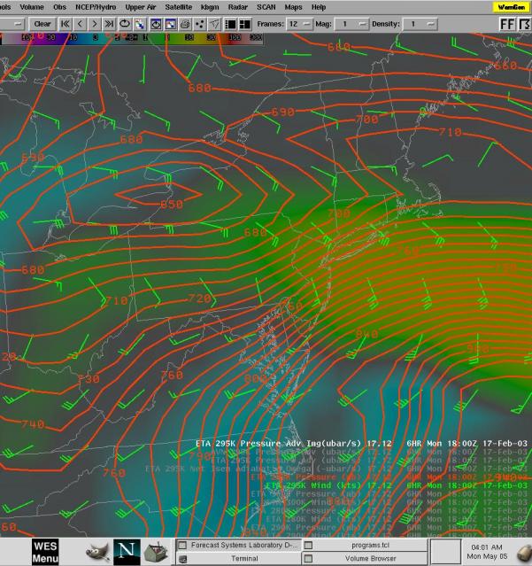
Figure 13a. 6-hour Eta forecast of wind and pressure
(red lines) and pressure advection (image)
on the 295 K isentropic surface verifying at 1800 UTC on the 17th.
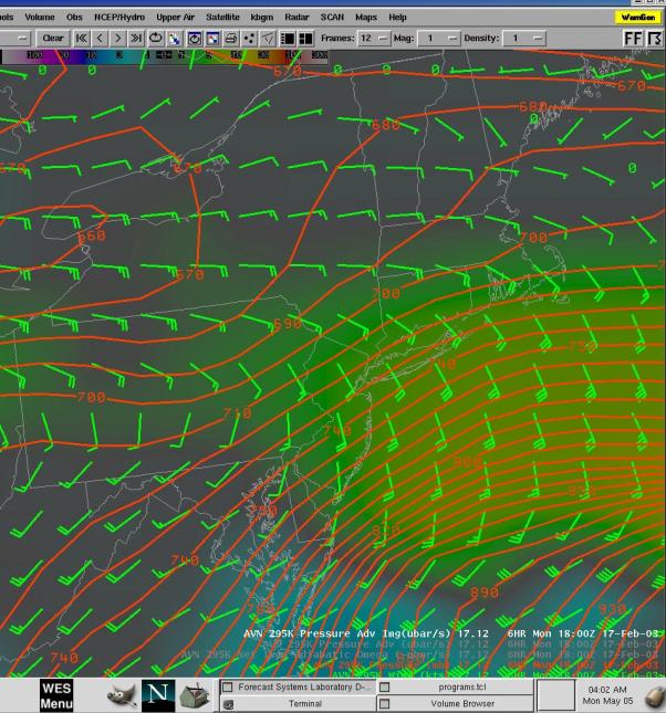
Figure 13b. 6-hour GFS
forecast of wind and pressure (red lines) and pressure advection
(image) on the 295 K isentropic surface
verifying at 1800 UTC on the 17th.
The stronger low-level easterly flow from the Eta forecasts, along with a stronger Eta pressure gradient result in stronger pressure advection and more implied upward motion over northeast Pennsylvania and southern New York in the Eta forecast. The stronger pressure gradient indicates that theta surfaces were sloped more steeply in the Eta forecast, implying a stronger temperature gradient. A comparison of temperatures on constant pressure surfaces between the Eta and GFS (not shown) confirms that the Eta forecast a stronger temperature gradient over eastern Pennsylvania and southern New York than the GFS.
- Summary.
A significant
snowstorm occurred over northeast Pennsylvania and central New York on the 17th,
despite the fact that the associated surface low-pressure center only deepened
to 1008 mb off of the mid-Atlantic coast.
In this case, heavy snow fell in association with a strong low-level
easterly jet (with speeds exceeding 50 kts).
The low-level jet developed as the lower-part of a strong circulation
driven by 1) strong large-scale forcing associated with upper-level vorticity
advection, and 2) strong mid-level frontogenesis. The Eta had a heavier, more accurate precipitation forecast than
the GFS with this event. Possible
reasons for the Eta’s better performance include a better depiction of a strong
short-wave ridge over New England (and resultant stronger upper-level vorticity
advection), a better depiction of a strong low-level easterly jet, and possibly
a better depiction of the low-level temperature structure of the atmosphere.